Contents
% To begin, add '$(TOOLBOX_PATH)/matlab' to the library path. The
% environment variable TOOLBOX_PATH needs to be set to the base
% directory of the reconstruction tools package.

if isempty(getenv('TOOLBOX_PATH'))
	error('Environment variable TOOLBOX_PATH is not set.');
end

addpath(strcat(getenv('TOOLBOX_PATH'), '/matlab'));
ESPIRiT examples (based on work by Sana Vaziri)
The input and output datasets are each stored in a pair of files: one header (.hdr) and one raw data (.cfl). All the data files used in this demo are in the data folder. The readcfl and writecfl Matlab methods can be found in $(TOOLBOX_PATH)/matlab and can be used to view and process the data and reconstructed images in Matlab.
Example 1: ESPIRiT reconstruction (R = 2x2)
The example uses ESPIRiT to obtain the image from 2x2 undersampled data.
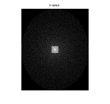
A visualization of k-space data and sampling and zero-filled reconstruction
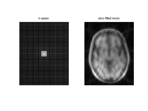
% sqrt sum-of-squares of k-space
und2x2 = readcfl('data/und2x2');
ksp_rss = bart('rss 8', und2x2);

% zero-filled reconstruction sqrt-sum-of-squares
zf_coils = bart('fft -i 6', und2x2);
zf_rss = bart('rss 8', zf_coils);

ksp_rss = squeeze(ksp_rss);
zf_coils = squeeze(zf_coils);
zf_rss = squeeze(zf_rss);

figure,subplot(1,2,1), imshow(abs(ksp_rss).^0.125, []); title('k-space')
subplot(1,2,2), imshow(abs(zf_rss), []); title('zero-filled recon')
Show singular values of the calibration matrix
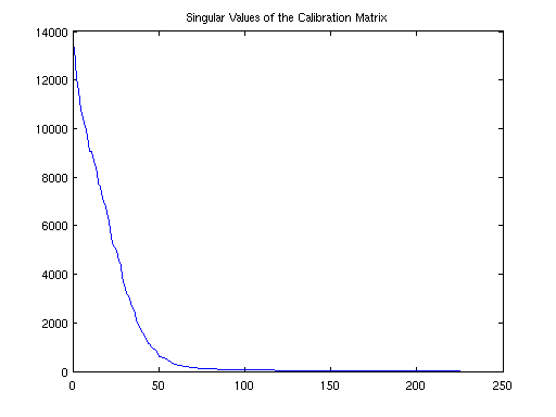
calmat = bart('calmat -r 20 -k 6', und2x2);
[U SV VH] = bart('svd', calmat);

figure, plot(SV);
title('Singular Values of the Calibration Matrix');
ESPIRiT calibration (using a maximum calibration region of size 20)
[calib emaps] = bart('ecalib -r 20', und2x2);
Calibration region...  (size: 1x20x20, pos: 0x105x80)
Energy: 0.568 0.282 0.104 0.031 0.008 0.003 0.002 0.001
Build calibration matrix and SVD...
Eigen decomposition... (size: 288)
Using 56/288 kernels (19.44%, last SV: 0.031736).
Zeropad...
FFT (juggling)...
Calculate Gram matrix...
Resize...
Point-wise eigen-decomposition...
Crop maps... (0.80)
Fix phase...
Done.
Extraction of first set of maps (0-th subarray along dimension 4)
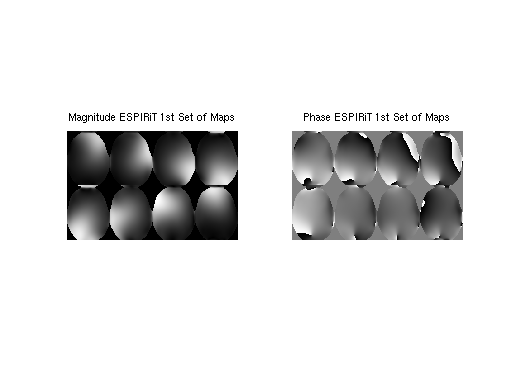
sens = bart('slice 4 0', calib);


sens_maps = squeeze(sens);

figure,
subplot(121), imshow3(abs(sens_maps), [],[2,4]);
title('Magnitude ESPIRiT 1st Set of Maps')
subplot(122), imshow3(angle(sens_maps),[],[2,4])
title('Phase ESPIRiT 1st Set of Maps')
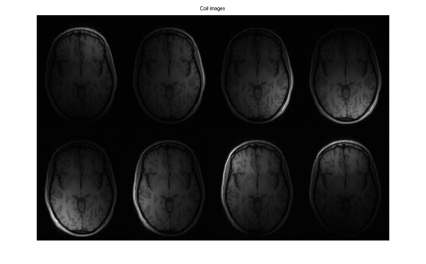
For comparison: Produce coil images from fully-sampled data using the fft command. It uses a bitmask as argument to specify the dimensions which are transformed. Here, the bitmask is 6 = 2^1 + 2^2 which corresponds to the dimensions 1 and 2.
full = readcfl('data/full');
coilimgs = bart('fft -i 6', full);

coil_imgs = squeeze(coilimgs);
figure, imshow3(abs(coil_imgs), [],[2,4])
title('Coil images')
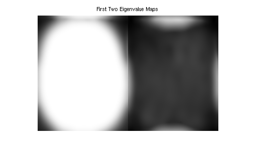
Show eigenvalue maps
emaps = squeeze(emaps);
figure, imshow3(emaps, [], [1, 2]);
title('First Two Eigenvalue Maps')
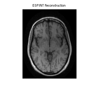
SENSE reconstruction using ESPIRiT maps (using the generalized parallel imaging compressed sensing tool)
reco = bart('pics', und2x2, sens);

sense_recon = squeeze(reco);
figure, imshow(abs(sense_recon), []); title('ESPIRiT Reconstruction')
Size: 41400 Samples: 10650 Acc: 3.89
l2 regularization: 0.000000
conjugate gradients
Total Time: 0.652066
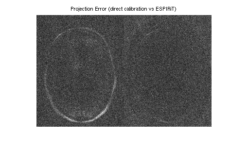
Evaluation of the coil sensitivities.
%
% Computing error from projecting fully sampled error
% onto the sensitivities. This can be done with one
% iteration of POCSENSE.
%
proj = bart('pocsense -r 0. -i 1', full, sens);

% Compute error and transform it into image domain and combine into a single map.
errimgs = bart('fft -i 6', (full - proj));
errsos_espirit = bart('rss 8', errimgs);

%
% For comparison: compute sensitivities directly from the center.
sens_direct = bart('caldir 20', und2x2);

% Compute error map.
proj = bart('pocsense -r 0. -i 1', full, sens_direct);
errimgs = bart('fft -i 6', (full - proj));
errsos_direct = bart('rss 8', errimgs);


errsos_espirit = squeeze(errsos_espirit);
errsos_direct = squeeze(errsos_direct);

figure,
imshow(abs([errsos_direct errsos_espirit]), []); title('Projection Error (direct calibration vs ESPIRiT)');
Reconstruction...
Done
Done.
Calibration region 1x20x20
Done.
Reconstruction...
Done
Done.
Example 2: Reconstruction of undersampled data with small FOV.
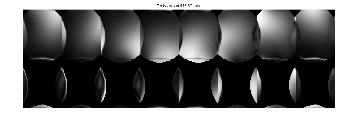
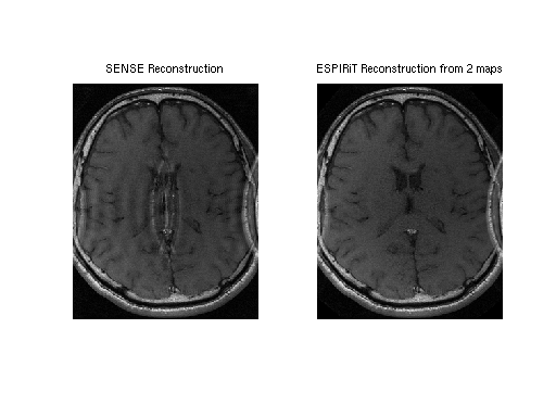
This example uses a undersampled data set with a small FOV. The image reconstructed using ESPIRiT is compared to an image reconstructed with SENSE. By using two sets of maps, ESPIRiT can avoid the central artifact which appears in the SENSE reconstruction.
% Zero padding to make square voxels since resolution in x-y for this
% data set is lower in phase-encode than readout
smallfov = readcfl('data/smallfov');
smallfov = bart('resize -c 2 252', smallfov);

% Direct calibration of the sensitivities from k-space center for SENSE
sensemaps = bart('caldir 20', smallfov);

% SENSE reconstruction
sensereco = bart('pics -r0.01', smallfov, sensemaps);

% ESPIRiT calibration with 2 maps to mitigate with aliasing in the calibration
espiritmaps = bart('ecalib -r 20 -m 2', smallfov);

% ESPIRiT reconstruction with 2 sets of maps
espiritreco = bart('pics -r0.01', smallfov, espiritmaps);

% Combination of the two ESPIRiT images using root of sum of squares
espiritreco_rss = bart('rss 16', espiritreco);

espirit_maps = squeeze(espiritmaps);
figure, imshow3(abs(espirit_maps), [],[2,8])
title('The two sets of ESPIRiT maps')
Calibration region 1x20x20
Done.
Size: 80640 Samples: 27167 Acc: 2.97
l2 regularization: 0.010000
conjugate gradients
Total Time: 0.630694
Calibration region...  (size: 1x20x20, pos: 0x150x116)
Energy: 0.515 0.306 0.115 0.045 0.013 0.004 0.002 0.001
Build calibration matrix and SVD...
Eigen decomposition... (size: 288)
Using 73/288 kernels (25.35%, last SV: 0.034163).
Zeropad...
FFT (juggling)...
Calculate Gram matrix...
Resize...
Point-wise eigen-decomposition...
Crop maps... (0.80)
Fix phase...
Done.
2 maps.
ESPIRiT reconstruction.
Size: 80640 Samples: 27167 Acc: 2.97
l2 regularization: 0.010000
conjugate gradients
Total Time: 0.682624
Warning: Image is too big to fit on screen; displaying at 50%
% SENSE image:

reco1 = squeeze(sensereco);
figure,
subplot(1,2,1), imshow(abs(reco1), [])
title('SENSE Reconstruction')


% ESPIRiT image:

reco2 = squeeze(espiritreco_rss);
subplot(1,2,2), imshow(abs(reco2), [])
title('ESPIRiT Reconstruction from 2 maps')
Example 3: Compressed Sensing and Parallel Imaging
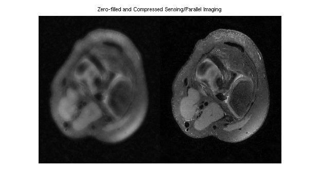
This example demonstrates L1-ESPIRiT reconstruction of a human knee. Data has been acquired with variable-density poisson-disc sampling.
% A visualization of k-space data

knee = readcfl('data/knee');
ksp_rss = bart('rss 8', knee);

ksp_rss = squeeze(ksp_rss);
figure, imshow(abs(ksp_rss).^0.125, []); title('k-space')


% Root-of-sum-of-squares image

knee_imgs = bart('fft -i 6', knee);
knee_rss = bart('rss 8', knee_imgs);


% ESPIRiT calibration (one map)

knee_maps = bart('ecalib -c0. -m1', knee);


% l1-regularized reconstruction (wavelet basis)

knee_l1 = bart('pics -l1 -r0.01', knee, knee_maps);


% Results

knee_rss = knee_rss / 1.5E9;

image = [ squeeze(knee_rss) squeeze(knee_l1) ];
figure, imshow(abs(image), [])
title('Zero-filled and Compressed Sensing/Parallel Imaging')
Calibration region...  (size: 1x24x24, pos: 0x132x106)
Energy: 0.560 0.266 0.116 0.037 0.010 0.006 0.004 0.001
Build calibration matrix and SVD...
Eigen decomposition... (size: 288)
Using 61/288 kernels (21.18%, last SV: 0.032264).
Zeropad...
FFT (juggling)...
Calculate Gram matrix...
Resize...
Point-wise eigen-decomposition...
Crop maps... (0.00)
Fix phase...
Done.
Size: 67968 Samples: 8082 Acc: 8.41
l1-wavelet regularization: 0.010000
FISTA
Total Time: 5.277991
Example 4: Basic Tools
Various tools are demonstrated by manipulating an image.
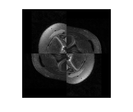
knee_l1 = readcfl('data/knee_l1');

% Zero pad

knee2 = bart('resize -c 1 300 2 300', knee_l1);

% Switch dimensions 1 and 2

tmp = bart('transpose 1 2', knee2);

% Scale by a factor of 0.5

tmp2 = bart('scale 0.5', tmp);

% Join original and the transposed and scaled version along dimension 2.

joined = bart('join 2', knee2, tmp2);

% Flip 1st and 2nd dimension (2^1 + 2^2 = 6)

tmp = bart('flip 6', joined);

% Join flipped and original along dimension 1.

big = bart('join 1', joined, tmp);

% Extract sub-array

tmp = bart('extract 1 150 449', big);
small = bart('extract 2 150 449', tmp);

% Circular shift by 115 pixels

tmp = bart('circshift 1 150', small);
shift = bart('circshift 2 150', tmp);

% Show the final result.

figure, imshow(abs(squeeze(shift)), []);
non-Cartesian MRI using BART
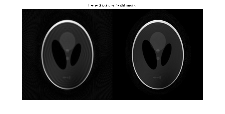
% Generate k-space trajectory with 64 radial spokes
traj_rad = bart('traj -r -x512 -y64');

% 2x oversampling
traj_rad2 = bart('scale 0.5', traj_rad);

% simulate eight-channel k-space data
ksp_sim = bart('phantom -k -s8 -t', traj_rad2);

% increase the reconstructed FOV a bit
traj_rad2 = bart('scale 0.6', traj_rad);


% inverse gridding
igrid = bart('nufft -i -t', traj_rad2, ksp_sim);

% channel combination
reco1 = bart('rss 8', igrid);


% reconstruct low-resolution image and transform back to k-space
lowres_img = bart('nufft -i -d24:24:1 -t', traj_rad2, ksp_sim);
lowres_ksp = bart('fft -u 7', lowres_img);

% zeropad to full size
ksp_zerop = bart('resize -c 0 308 1 308', lowres_ksp);

% ESPIRiT calibration
sens = bart('ecalib -m1', ksp_zerop);

% non-Cartesian parallel imging
reco2 = bart('pics -S -r0.001 -t', traj_rad2, ksp_sim, sens);


figure, imshow(abs(squeeze([reco1, reco2])), []);
title('Inverse Gridding vs Parallel Imaging')
Est. image size: 308 308 1
Done.
Done.
Calibration region...  (size: 24x24x1, pos: 142x142x0)
Energy: 0.591 0.287 0.102 0.015 0.004 0.001 0.000 0.000
Build calibration matrix and SVD...
Eigen decomposition... (size: 288)
Using 38/288 kernels (13.19%, last SV: 0.037886).
Zeropad...
FFT (juggling)...
Calculate Gram matrix...
Resize...
Point-wise eigen-decomposition...
Crop maps... (0.80)
Fix phase...
Done.
l2 regularization: 0.001000
conjugate gradients
Total Time: 1.684765